Learning how to use the Network Analysis object
One of the most unique objects in SAS Visual Analytics might be the Network Analysis object, which is included with the base SAS Visual Analytics license.
Here you can display and dig into networks, how to customers relate to agents, who is my company internally structure, how are goods flowing through a system. But using the object was never straight forward to me, so lets explore it together.
Note: we will be jumping into SAS Studio from time to time to create data which we will use in our exploration - these will be highlighted through Stop Studio Time.
As always the basis for my learning is of course the SAS Documentation which I recommend you also check out.
You can find the SAS code for this blog post here and if you want to import the SAS Visual Analytics report using SAS Environment Manager, you can find the JSON for that here.
There is also an interactive audio visual experience that you can check out over here.
Intro
The Network Analysis object visualizes relationships between data values through interconnected nodes. Two types of network analyses can be created: Hierarchical, which organizes data using a hierarchy, and Ungrouped, which establishes connections between a source and target data item.
You can find the Network Analysis object in the Objects pane in the category Analytics. When you drag and drop this object into a report the default network structure is Ungrouped, because of that we will also start of our journey with the ungrouped network.
Note: a lot of the Options and Roles are shared between both the Ungrouped and the Hierarchical networks, so they will only be explained in the Ungrouped chapter.
Ungrouped
The ungrouped network structure can help us visualize structures within our data of which we currently are unsure how they relate or group together. The Network Analysis object with the ungrouped network structure requires only two data items. The two data items have to be classified as Category and have to have the same data type, i.e. both numeric or both character. The two required items are Source and Target. The Source contains the data for all of the nodes that will be displayed in the network. The Target contains the data to create the links between nodes.
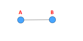
Before we actually go and build our first network let us consider the previous paragraph with the simplest possible network. This network has just two nodes A and B and they are connected by a link:
Now how this network look like if we translate it into a table - First we would need our Source column which contains two entries A and B, next we need a second column Target that contains the link between A and B, please note I left how the link type on purpose here as it is a concept we will tackle later on. So to make it easy on ourselves we can just enter B and A into the column to get the final table:
| Source | Target |
|---|---|
| A | B |
| B | A |
Now we could assign the Source column as our Source data item and analogous for the Target, to get the above network, but that isn't really that interesting now is it? So let's get into some more interesting data.
Note: if the Source and Target data items are Geographical then the Network Analysis object will be converted into a Geo Network object.
Basic Setup
Stop Studio Time - the following code will generate a very small table into your casuser library called Employees which will contain our first example data, please run it and then add the data to a new SAS Visual Analytics report.
cas mysess;

* Quietly dropping the table so you can always rerun this code;
proc casutil;
    droptable incaslib='casuser' casdata='Employees' quiet;
quit;

* This example data can be found in the SAS Documentation;
data casuser.Employees(promote=yes);
   input Employee $ Manager $ Salary EmployeeID ManagerID;
   datalines;
EMP1 MGR1 40000 2 1
EMP2 MGR1 55000 3 1
EMP3 MGR1 50000 4 1
MGR1 . 75000 1 .
;
run;
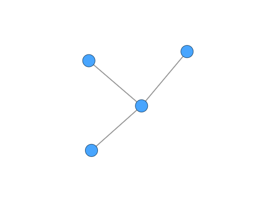
When you look into the Data pane you will see that you first have to convert the EmployeeID and ManagerID to categories to make use of them in the Network Analysis object. Here you have to make a decision, do you want to use the numeric ID or the actual text. I will be choosing the the actual text variable (Employee & Manager) but it works analogous. Our first ungrouped network will look like this:
To the Options
Now that we have created our very first and very basic network, let us explore the Options pane of the object for a bit. We will be skipping the standard sections like Object, Style and Graph Frame and rather work our way through the sections Network Analysis and Network Display.
The Network Analysis section contains only the General heading. Here we have one that we have already talked about quite a bit Network structure. As you can see the default is set to Ungrouped, the second value that is available is Hierarchical for which there is an additional section in this document. So let's take a look at the second option available to us Link type. Here the default is set to Undirected and if we change it to Directed, seemingly nothing happens in our graph. But there is things happening behind the scenes, let us talk about that first what is meant by Undirected first. Undirected means that the links between nodes are bidirectional meaning there is a two-way relationship between the nodes, for example think of a typical street which you can drive down in both directions. Now the Directed link type defines that there is a clear relationship in one-way, think of a one-way street which cars are only allowed to drive down in one direction. Our example is very directed all of the Employees work for that one Manager, except for our poor manager who works for missing. So what is effected by changing Link type, first if we activate the Link arrows option we see a drastic change, will take a look at that soon, and second it affects the calculation of network metrics (for more on these please see the section Network Metrics).
Next we will move to the Network Display section which contains five headings:
- Network Diagram: Gives you the ability to Abbreviate numeric values (as usual you can adjust the Scale and the Digits of precision), enable Data labels (this displays the source text of the node or the Hierarchical level of the node or if you specify a Label as role, then that value is used instead), enable Link arrows (this will show arrow heads on the links, here the Link type option becomes very important), enable Detailed link attributes (displayed every link between each node pair, by default they are aggregated) and set the amount Link curvature (this curves the link between nodes and can help make the diagram feel more dynamic)
- Network Layout: Gives you the ability to change the Node size (how big is the node in the diagram), adjust the Force strength (adjust the positions of nodes and links, in general bigger values lead to more space between nodes - not available with Map background enabled) and Node distance (adjust the distance between nodes, in general bigger values lead to more space between nodes - not available with Map background enabled). The reason for the Force strength and Node distance not being available if you have a Map background is because the layout is then tied to that geographic map and adjusting these options would lead to distortions
- Node Selection: Ability to define how many Predecessors (only if the Link type is set to Directed) and Successors that are selected. This option is only available if you select a node in the diagram, then right click it, go to Selection and click on Set as source for selection
- Map: If you have data items that are classified as Geography (this applies to Source and Target and Levels for the Hierarchical network), then your object is automatically moved to the Geo network object (which can be found in the Objects pane under the Geo Maps section) and a Map background can be applied, a Map services can be selected and the Transparency can be adjusted
- Legend: This heading should be familiar from other SAS Visual Analytics objects and doesn't offer any specific additional options for the Network Analysis object
To the Roles
Besides the Source and Target role we have already explored, but in addition we have six optional roles that we can make use of:
- Size, influences the actual size of each node relative to other nodes, the internal metrics Reach Centrality, Closeness Centrality and Betweenness Centrality can be used here, can only be a Measure
- Color, changes the color of each node, the internal metrics Reach Centrality, Closeness Centrality, Betweenness Centrality, Community and Disconnected Network ID can be used here, can be a Category, Geography or Measure - Note: this overwrites any Display Rules that might have been applied to the object
- Link width, can only be a Measure - if assigned the value will be added as a Data tip value when hovering over the link between nodes
- Link color, determines the color of the link between nodes, can be a Category, Geography or Measure - if assigned the value will be added as a Data tip value when hovering over the link between nodes
- Label, the value is displayed if the Data labels option is enabled, can be a Category, Geography or Measure
- Data tip values, displayed additional information when hovering over a node, can be a Category, Geography or Measure
Actions, Display Rules, Filters and Ranks
This guide will note dig into these additional Panes as there is nothing really specific about Networks Analysis objects when it comes to these panes.
Maximizing the Object
When you go to a Network Analysis object and click the Maximize icon, you will see two tabs coming up. The first will be named Network - name of the data item Source/Levels, it contains a detailed table of information about the network - especially interesting is the Item Type, which can be Node or Link, in combination with the Source and Target columns. The second tab is the Network Analysis Summary, which contains a generated natural language explanation of the displayed network.
Working with the Geographic Features
There are a lot of capabilities packed into the geographic side of things, like searching, pinning, areas, additional statistics, routes, etc. - as this would be more of a dive into Geo Maps objects, I am not going to go into this further, but rather point you towards the SAS Documentation at this point.
Selection
You can select network nodes and then right click your selection to calculate the Shortest path between the nodes. You can also select the Largest cluster or the Smallest cluster, etc. To find out more about the available Selections check out the SAS Documentation.
Hierarchical
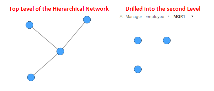
If we change the Network structure from its default value to Hierarchical, we have to go to the Roles pane and change things up. The Source and Target roles are gone in favor of the new Levels role. The Levels role requires a Date item of the type Hierarchy, which you can create via the New data item in the Data pane. Each level of the Hierarchy corresponds to the level when you drill (double click) into nodes. If your Hierarchy is a Geographical Hierarchy, then your Network Analysis object is automatically converted into a Geo Network object (this enables the Map option in the Options pane).
Working of the base example provided above, we can create a new Hierarchy data item Manager - Employee by first adding the Manager and then the Employee. Next we add a new Network Analysis object, change the Network structure to Hierarchical and assign our new Hierarchy to the Levels role:
To the Options
With the Hierarchical network structure we have some additional options available to use.
In the Network Analysis section under the General heading you can find the additional option Additional levels. This options adjusted how many levels of the hierarchy are displayed in addition to the currently selected level. If we stick to the base example where we have Manager - Employee hierarchy if we set the Additional levels to 0 we would only see two nodes in our network (missing and MGR1), only when drilling into a node would we see what is underneath, but when we set the level to 1 we would see the full network be displayed (MGR1, missing and MGR1, EMP1, EMP2, EMP3):
Actions, Display Rules, Filters and Ranks
When you switch to the Hierarchical network structure you limit the amount of actions that can be applied to the object - now only the Automatic actions on all objects option can be used.
Network Metrics
The Network Analysis object generates five additional metrics internally that can be used to customize the roles of the object. These metrics can be used as variables in the Size and/or Color roles. Let us quickly talk about them:
- Reach Centrality, can be used both as Size and Color, indicates how many links away the farthest connect link is, this leads to nodes in the center to have small values. It quantifies how efficiently information can spread from a given node to other nodes in the network
- Closeness Centrality, can be used both as Size and Color, indicates how close a node is to all of its connected nodes, this leads to nodes in the center to have high values. A higher closeness centrality value implies that a node can efficiently interact with other nodes in the network
- Betweenness Centrality, can be used both as Size and Color, indicates how often a given node is part of the shortest path between nodes. Nodes with high betweenness centrality act as bridges or intermediaries between different parts of the network. They have significant control over information flow because a large proportion of shortest paths between other nodes pass through them. Nodes with high betweenness centrality play a crucial role in maintaining connectivity and facilitating communication between disparate parts of the network
- Community, can be used only as Color, identifies local groupings of nodes. The community measure in network analytics aims to uncover meaningful structures or groups within a network, revealing nodes that share stronger connections among themselves compared to nodes in other parts of the network (if the Detailed link attributes option is enables it can influence the calculation)
- Disconnected Network ID, can be used only as Color, is an ID that is assigned to disjointed or disconnected components with a network. It serves as a marker to quickly distinguish between the disconnected parts of a network and can help to understand different relationships and properties
If you add the Community metric to the Color role then you can go to the Options pane and under the heading General in the section Network Analysis you will find the additional option Community resolution. This option influences the number and size of communities that are identified. A Low resolution value results in large and generalized communities, while a High resolution tends towards smaller and more fine-grained communities. Playing with this parameter can help to identify different structures within a network, but note that we have a trade-off between granularity and interpretability for report consumers, you can adjust this parameter from Low (0) to High (1):
Extended Example
To play around with some additional features like Geo Network, URL Links and three level Hierarchy I have extended our base data set a bit - this doesn't break any thing from the original data set:
Stop Studio Time - run the following code:
cas mysess;

* Quietly dropping the table so you can always rerun this code;
proc casutil;
    droptable incaslib='casuser' casdata='Employees' quiet;
quit;

* This example data can be found in the SAS Documentation;
data casuser.Employees(promote=yes);
    length Link $512.;
   input Employee $ Manager $ Team $ Salary EmployeeID ManagerID Country $ State $ Link $;
   datalines;
EMP1 MGR1 A 40000 2 1 US NC https://go.documentation.sas.com/doc/en/vacdc/default/vaobj/n0kcvb9vm0kd1sn1b199uu8hgq1w.htm?requestorId=b499afb9-a7cb-4a66-b985-92b1fab6f3ee#n0r57nk56ysfnln1xd64od5b5s8i
EMP2 MGR1 A 55000 3 1 US NY https://go.documentation.sas.com/doc/en/vacdc/default/vaobj/n0kcvb9vm0kd1sn1b199uu8hgq1w.htm?requestorId=b499afb9-a7cb-4a66-b985-92b1fab6f3ee#n0zuutt5v6onehn1uuszwsvrpyl9
EMP3 MGR1 B 50000 4 1 US TX https://go.documentation.sas.com/doc/en/vacdc/default/vaobj/n0kcvb9vm0kd1sn1b199uu8hgq1w.htm?requestorId=b499afb9-a7cb-4a66-b985-92b1fab6f3ee#p0izq756yfu1syn177wdhj69ithm
MGR1 . . 75000 1 . US NC https://go.documentation.sas.com/doc/en/vacdc/default/vaobj/n0kcvb9vm0kd1sn1b199uu8hgq1w.htm?requestorId=b499afb9-a7cb-4a66-b985-92b1fab6f3ee#p09pqxhkq5urgin1vdqg93trlcgga
;
run;
Additional Resources
Great SAS Community article by Beth Ebersole, that also has a lot of additional resources linked - click here.
Want to learn more about the Community Detection, then checkout this SAS Documentation entry on the very topic.


